HSV 示例

此示例演示了 hsv 算子的用法，该算子操作图像的色调、饱和度和明度（亮度）方面。

简介

HSV 色彩空间

HSV 通过分离色调、饱和度和亮度来表示颜色。在此色彩空间中，色调表示为色轮上的一个角度。饱和度从 0（灰度）到 100%（完全饱和的颜色），值从 0（黑色）到 1（全亮度）。有关详细信息，请参阅：Wikipedia。

关于实现的说明

出于性能原因，DALI 没有使用 HSV 的精确定义，而是通过对 RGB 颜色进行线性（矩阵）运算来近似 HSV 空间中的运算。这大大提高了性能，但代价是适度损失了保真度。

步骤指南

1. 让我们从导入一些实用工具和 DALI 本身开始。

from nvidia.dali import pipeline_def
import nvidia.dali.fn as fn
import nvidia.dali.types as types

batch_size = 10
image_filename = "../data/images"

批大小大于一，以便于在笔记本末尾切换图像。

2. 接下来，让我们实现 pipeline。装饰函数 hsv_pipeline 可用于创建在 CPU 或 GPU 上处理数据的 pipeline，具体取决于 device 参数。

@pipeline_def()
def hsv_pipeline(device, hue, saturation, value):
    files, labels = fn.readers.file(file_root=image_filename)
    images = fn.decoders.image(
        files, device="cpu" if device == "cpu" else "mixed"
    )
    converted = fn.hsv(images, hue=hue, saturation=saturation, value=value)
    return images, converted

下面的函数用于实际显示 DALI 中 HSV 操作的结果。由于我们设置的 pipeline 返回 2 个输出：修改后的图像和原始图像，因此该函数从输出中获取两者并显示它们。指定了附加标志 (cpu)，以确定 pipeline 输出是来自 CPU 还是 GPU。在后一种情况下，我们必须告诉输出返回数据的 CPU 可访问副本。

import matplotlib.pyplot as plt
import matplotlib.gridspec as gridspec
import math


def display(outputs, idx, columns=2, captions=None, cpu=True):
    rows = int(math.ceil(len(outputs) / columns))
    fig = plt.figure()
    fig.set_size_inches(16, 6 * rows)
    gs = gridspec.GridSpec(rows, columns)
    row = 0
    col = 0
    for i, out in enumerate(outputs):
        plt.subplot(gs[i])
        plt.axis("off")
        if captions is not None:
            plt.title(captions[i])
        plt.imshow(out.at(idx) if cpu else out.as_cpu().at(idx))

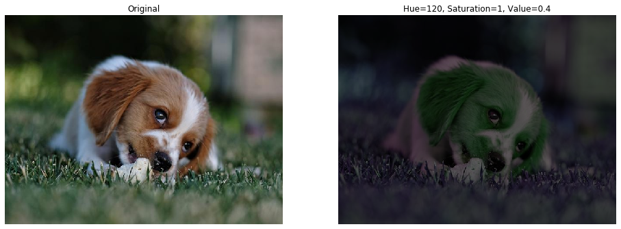
3. 现在让我们构建 pipeline，运行它们并显示结果。首先是 CPU pipeline

pipe_cpu = hsv_pipeline(
    device="cpu",
    hue=120,
    saturation=1,
    value=0.4,
    batch_size=batch_size,
    num_threads=1,
    device_id=0,
)
pipe_cpu.build()
cpu_output = pipe_cpu.run()

display(
    cpu_output, 3, captions=["Original", "Hue=120, Saturation=1, Value=0.4"]
)

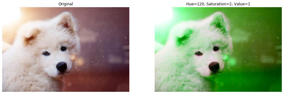
4. 以及 GPU

pipe_gpu = hsv_pipeline(
    device="gpu",
    hue=120,
    saturation=2,
    value=1,
    batch_size=batch_size,
    num_threads=1,
    device_id=0,
)
pipe_gpu.build()
gpu_output = pipe_gpu.run()

display(
    gpu_output,
    0,
    cpu=False,
    captions=["Original", "Hue=120, Saturation=2, Value=1"],
)

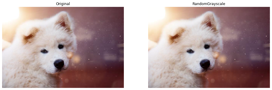
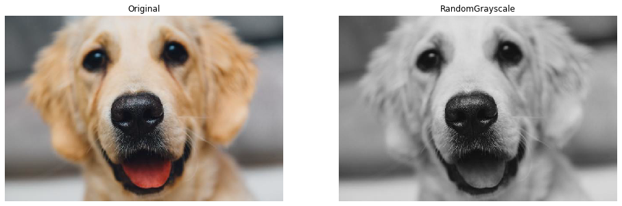
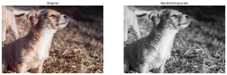
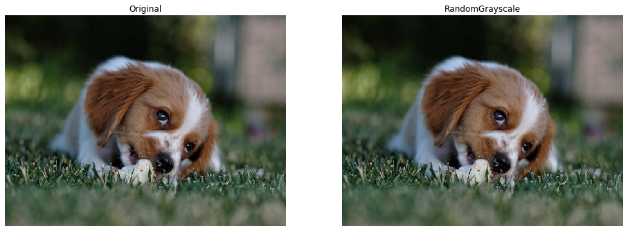
使用 HSV 实现 RandomGrayscale 操作

作为 Hsv 算子的一个更有趣的示例，我们希望实现类似于 Pytorch 的 RandomGrayscale 变换 - 对于 RGB 输入，将其转换为仍然包含 3 个通道（但值相等）的灰度图像，或者保持不变。

为了实现灰度转换，我们将降低输入的饱和度（将这些样本的 saturation 设置为 0）。如果我们将 saturation 设置为 1，则图像将保持其颜色。

我们可以使用 coin_flip 算子，该算子以可配置的概率返回 0 和 1。我们将使用 coin_flip 生成的值来驱动 hsv 算子的 saturation 参数。

coin_flip 为处理批次中的每个样本生成一个数字，我们可以将其传递给 hsv 中 saturation 参数。由于 coin_flip 返回整数，而 hsv 期望浮点数作为其参数，因此我们还需要使用 cast 转换这些值。

def random_grayscale(images, probability):
    saturate = fn.random.coin_flip(probability=1 - probability)
    saturate = fn.cast(saturate, dtype=types.FLOAT)
    return fn.hsv(images, saturation=saturate)


@pipeline_def(seed=422)
def random_grayscale_pipeline():
    files, labels = fn.readers.file(file_root=image_filename)
    images = fn.decoders.image(files, device="mixed")
    converted = random_grayscale(images, 0.6)
    return images, converted

现在让我们构建并运行 pipeline。

pipe = random_grayscale_pipeline(
    batch_size=batch_size, num_threads=1, device_id=0
)
pipe.build()
output = pipe.run()

display(output, 0, cpu=False, captions=["Original", "RandomGrayscale"])
display(output, 1, cpu=False, captions=["Original", "RandomGrayscale"])
display(output, 2, cpu=False, captions=["Original", "RandomGrayscale"])
display(output, 3, cpu=False, captions=["Original", "RandomGrayscale"])