pyAerial 中上行共享信道 (PUSCH) 的信道估计#
本笔记本为研究人员提供了一个关于如何在 pyAerial 中进行机器学习原型设计的示例。PyAerial 是 Aerial SDK 的 Python 绑定,Aerial SDK 是 NVIDIA 的 L1 和 L2 加速堆栈,也集成在 Aerial Omniverse Digital Twin (AODT) 中。这使研究人员能够开发符合标准的方法,专注于提高其链路级性能。随后,该方法可以在 AODT 中进行真实评估,展示链路级性能如何转化为系统级 KPI。
特别是,本笔记本侧重于改进基于 PUSCH 传输中 DMRS 导频的信道估计。首先,我们从 pyAerial PUSCH 管道中隔离信道估计器模块。信道估计是第一个接收器模块之一,如下图所示
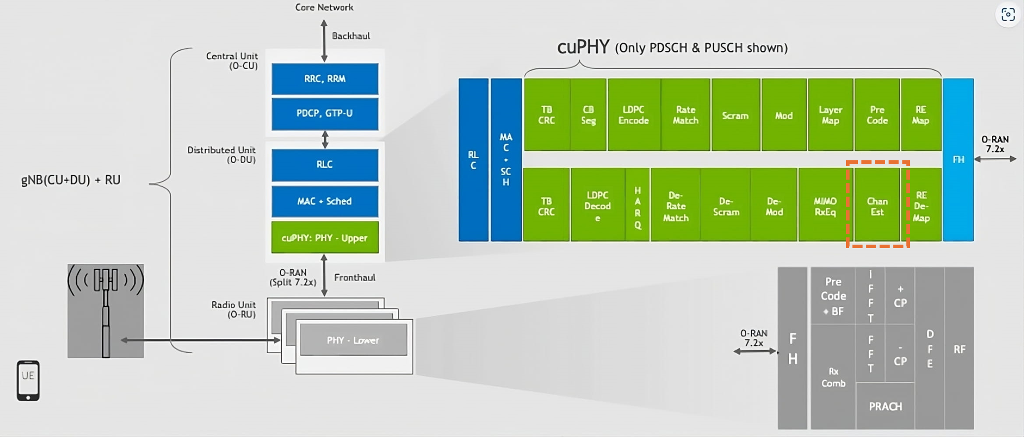
为了隔离信道估计模块,我们参考了 Example PUSCH Simulation.ipynb 中的模块化 PUSCH 管道。在那里,我们看到了如何将信道估计下游与资源元素 (RE) 解映射器和无线信道接口,以及上游与其他组件(如 MIMO 均衡器)接口。类似的方法可以用于接收器或发射器管道中的其他模块。
本笔记本使用 PyTorch 训练卷积神经网络,以改进和插值最小二乘 (LS) 信道估计。训练使用自定义 LS 估计器,该估计器与 Sionna 的资源网格、资源映射器和信道生成器接口。然后,将训练好的模型集成到 pyAerial PUSCH 管道中,并使用在 Sionna 信道之上运行的符合标准的信号传输和接收模块进行验证。
*
请参阅下文,了解我们如何训练和测试信道估计器模型。
[1]:
import os
# GPU setup
GPU_IDX = 2
os.environ["CUDA_VISIBLE_DEVICES"] = str(GPU_IDX)  # Select only one GPU
os.environ['TF_CPP_MIN_LOG_LEVEL'] = "3"  # Silence TensorFlow.

import torch
import numpy as np
from tqdm import tqdm
import tensorflow as tf
import matplotlib.pyplot as plt

# Our imports
from channel_gen_funcs import SionnaChannelGenerator
from channel_gen_funcs import PyAerialChannelEstimateGenerator
from channel_est_models import ChannelEstimator
from channel_est_models import ComplexMSELoss
import utils as ut

dev = torch.device(f'cuda')
torch.set_default_device(dev)

# General parameters
num_prbs = 48               # Number of PRBs in the UE allocated bandwidth
interp = 1                  # Interpolation factor. If 2, it estimates also for REs without DMRS
models_folder = f'saved_models_prbs={num_prbs}_interp={interp}' # Folder to save trained models

# Training parameters
train_snrs = np.array([10]) # Train models for these SNRs. Suggested: np.arange(-10, 40.1, 10)
training_ch_model = 'UMa'   # Channel model ['Rayleigh', 'CDL-x', 'TDL-x', 'UMa', 'UMi'],
                            # where x is in ["A", "B", "C", "D", "E"] as per TR 38.901
n_iter = 5000               # Number of training iterations. Best results: 30k
batch_size = 32             # Batch size = number of channels to train simultaneously
model_reuse = True          # Whether to load the weights of the last trained model
                            # (this trick improves convergence speed considerably)

# Testing parameters
test_snrs = np.arange(-10, 40.1, 5)  # Test models for these SNRs. Suggested: np.arange(-10, 40.1, 5)
testing_ch_model = 'UMi'             # Channel for testing
n_iter_test = 1000                   # Number of batches of channels to evaluate (batch=32)
[PhysicalDevice(name='/physical_device:GPU:0', device_type='GPU')]
训练信道估计模型#
示例机器学习模型使用最小二乘 (LS) 估计并输出更准确的信道估计。在其基本配置中,DMRS 在频率上具有 1/2 密度(即每两个子载波一个 RE)。因此,我们的 ChannelEstimator 可以输出与 DMRS 导频一样多的估计值(使用插值因子 interp=1 的一半子载波)或两倍的估计值(使用参数 interp=2),从而覆盖所有子载波。
关于训练的重要说明:我们的方法包括为每个 SNR 训练一个模型。特定于 SNR 的模型可以更准确地学习如何估计 SNR 接近用于模型训练的原始 SNR 的信道。此方法还解决了低 SNR 信道导致更高损耗并导致模型专注于它们而不适用于高 SNR 情况的问题。
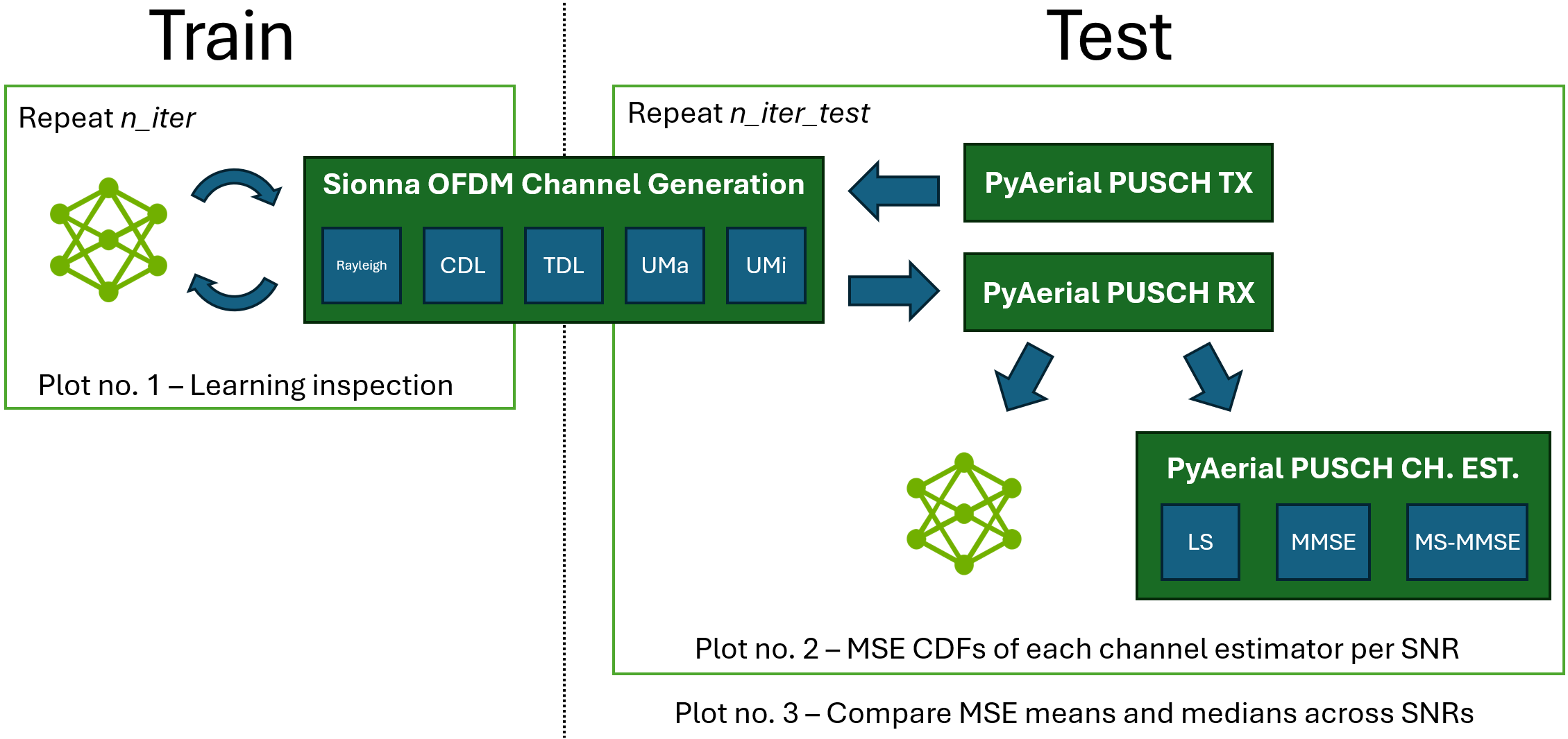
对于训练,模型直接与 Sionna 信道模型接口。对于测试,该模型集成在 pyAerial 的 PUSCH 管道中,并与其他经典信道估计器(如最小均方误差 (MMSE) 和多级 MMSE (MS-MMSE))一起进行评估。训练和测试的图表如下
[2]:
models_dir = ut.get_model_training_dir(models_folder, training_ch_model,
num_prbs, n_iter, batch_size)
os.makedirs(models_dir, exist_ok=True)
# Channel generator for training
train_ch_gen = SionnaChannelGenerator(num_prbs, training_ch_model, batch_size)
last_model = ''
for snr_idx, snr in enumerate(train_snrs):
print(f'Training model for SNRs: {snr} dB')
save_model_path = ut.get_snr_model_path(models_dir, snr)
model = ChannelEstimator(num_prbs*12//2, freq_interp_factor=interp).to(dev)
reload_last_model = model_reuse and last_model
if reload_last_model:
model.load_state_dict(torch.load(last_model))
criterion = ComplexMSELoss()
optimizer = torch.optim.AdamW(model.parameters(), lr=1e-3, weight_decay=1e-4)
model.train()
train_loss, mse_loss = [], []
count = []
for i in (pbar := tqdm(range(n_iter // (5 if reload_last_model else 1)))):
h, h_ls = train_ch_gen.gen_channel_jit(snr)
# Transition tensors to PyTorch for learning
h, h_ls = torch.tensor(h.numpy()).to(dev), torch.tensor(h_ls.numpy()).to(dev)
# Uncomment to inspect estimates vs ground-truth channel
# ut.compare_ch_ests([h_ls.cpu().numpy()[0,:], h.cpu().numpy()[0,:]],
# ['LS', 'GT'], title=f'SNR = {snr} dB')
h_hat = model(h_ls[..., ::2])
loss = criterion(h_hat, h[..., ::(3-interp)])
optimizer.zero_grad(); loss.backward(); optimizer.step()
train_loss += [ut.db(loss.item())]
pbar.set_description(f"Iteration {i+1}/{n_iter}")
pbar.set_postfix_str(f"Training loss: {train_loss[-1]:.1f} dB")
last_model = save_model_path
torch.save(model.state_dict(), save_model_path)
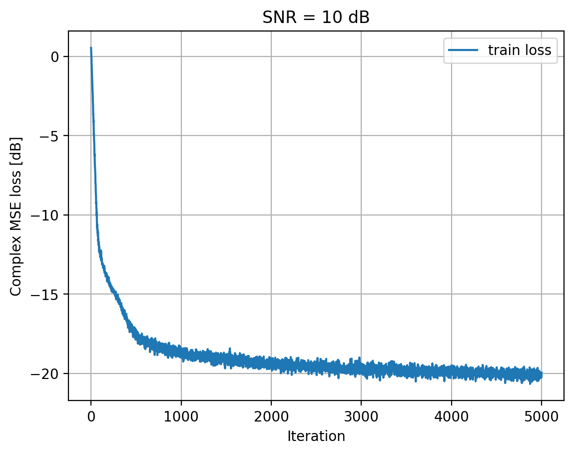
ut.plot_losses([train_loss], ['train loss'], title=f'SNR = {snr} dB')
XLA can lead to reduced numerical precision. Use with care.
Training model for SNRs: 10 dB
  0%|                                                                                                                              | 0/5000 [00:00<?, ?it/s]WARNING: All log messages before absl::InitializeLog() is called are written to STDERR
I0000 00:00:1729133880.135412    9045 device_compiler.h:186] Compiled cluster using XLA!  This line is logged at most once for the lifetime of the process.
Iteration 5000/5000: 100%|████████████████████████████████████████████████████████████████████| 5000/5000 [00:49<00:00, 101.48it/s, Training loss: -20.0 dB]
测试信道估计模型#
上面训练的模型是一个深度卷积网络,由 RESNET 层组成,如果启用插值 (interp = 2),则可能在末尾有一个全连接层。下面给出了此网络的图,以分配 48 个 PRB 的示例用户为例
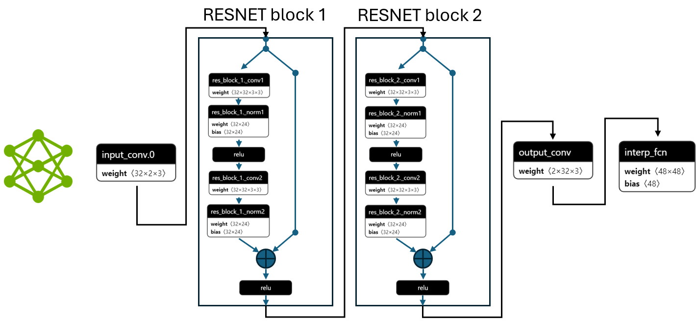
现在,我们使用从 PUSCH 接收器提取的 LS 信道估计来评估此网络,而不是手动从信道中提取。网络的输出与 MS-MMSE 进行比较。
[3]:
train_dir = ut.get_model_training_dir(models_folder, training_ch_model,
num_prbs, n_iter, batch_size)
snr_losses_ls = [] # Least Squares channel estimation losses
snr_losses_ml = [] # Machine learning channel estimation losses
snr_losses_ml2 = [] # Machine learning channel estimation losses (median)
snr_losses_ls_pyaerial = [] # LS from PyAerial
snr_losses_mmse_pyaerial = [] # MMSE from PyAerial
snr_losses_mmse_pyaerial2 = [] # MMSE from PyAerial (median)
# Channel generator for testing
test_ch_gen = SionnaChannelGenerator(num_prbs, testing_ch_model, batch_size=32)
# Create pyAerial channel estimate generator, using the Sionna Channel Generator
pyaerial_ch_est_gen = PyAerialChannelEstimateGenerator(test_ch_gen)
for snr_idx, snr in enumerate(test_snrs):
print(f'Testing SNR {snr} dB')
# Select model trained on the SNR closest to the test SNR
snr_model_idx = np.argmin(abs(train_snrs - snr))
snr_model = train_snrs[snr_model_idx]
print(f'Testing model trained on SNR {snr_model}')
# Load ML model
model = ChannelEstimator(num_prbs*12//2, freq_interp_factor=interp).to(dev)
model.load_state_dict(torch.load(ut.get_snr_model_path(train_dir, snr_model)))
criterion = ComplexMSELoss()
model.eval()
ls_loss, ml_loss, ls_loss_pyaerial, mmse_loss_pyaerial = [], [], [], []
with torch.no_grad():
for i in tqdm(range(n_iter_test), desc='Testing LS & MS-MMSE in PyAerial'):
# Internally generate channels, add noise, receive the DM-RS symbols and estimate the channel
ls, mmse, gt = pyaerial_ch_est_gen(snr)
# Evaluate pyAerial classic estimators
for b in range(len(ls)):
ls_loss_pyaerial += [ut.complex_mse_loss(ls[b], gt[b][::2])]
mmse_loss_pyaerial += [ut.complex_mse_loss(mmse[b], gt[b])]
# Evaluate ML approach
h, h_ls = torch.tensor(gt).to(dev), torch.tensor(ls).to(dev)
h_hat = model(h_ls) # h_ls has half the subcarriers of h already
ls_loss += [criterion(h_ls, h[..., ::2]).item()]
ml_loss += [criterion(h_hat, h[..., ::(3-interp)]).item()]
# Compute means and medians of LS, LS+ML and MS-MMSE
snr_losses_ls += [ut.db(np.mean(ls_loss))]
snr_losses_ml += [ut.db(np.mean(ml_loss))]
snr_losses_ml2 += [ut.db(np.median(ml_loss))]
snr_losses_ls_pyaerial += [ut.db(np.mean(ls_loss_pyaerial))]
snr_losses_mmse_pyaerial += [ut.db(np.mean(mmse_loss_pyaerial))]
snr_losses_mmse_pyaerial2 += [ut.db(np.median(mmse_loss_pyaerial))]
print(f'Avg. ML test loss for {snr} dB SNR is {snr_losses_ml[-1]:.1f} dB')
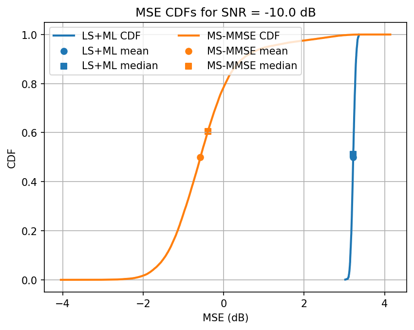
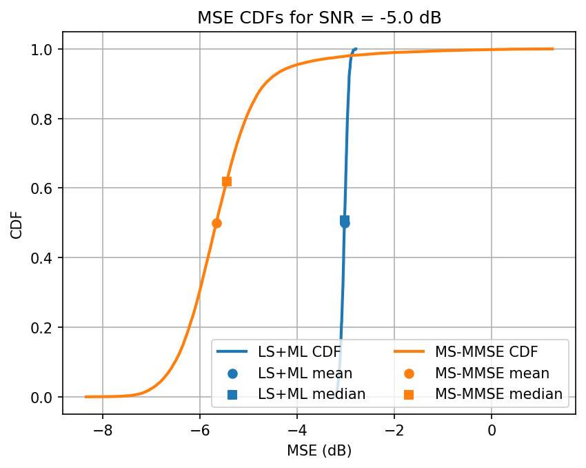
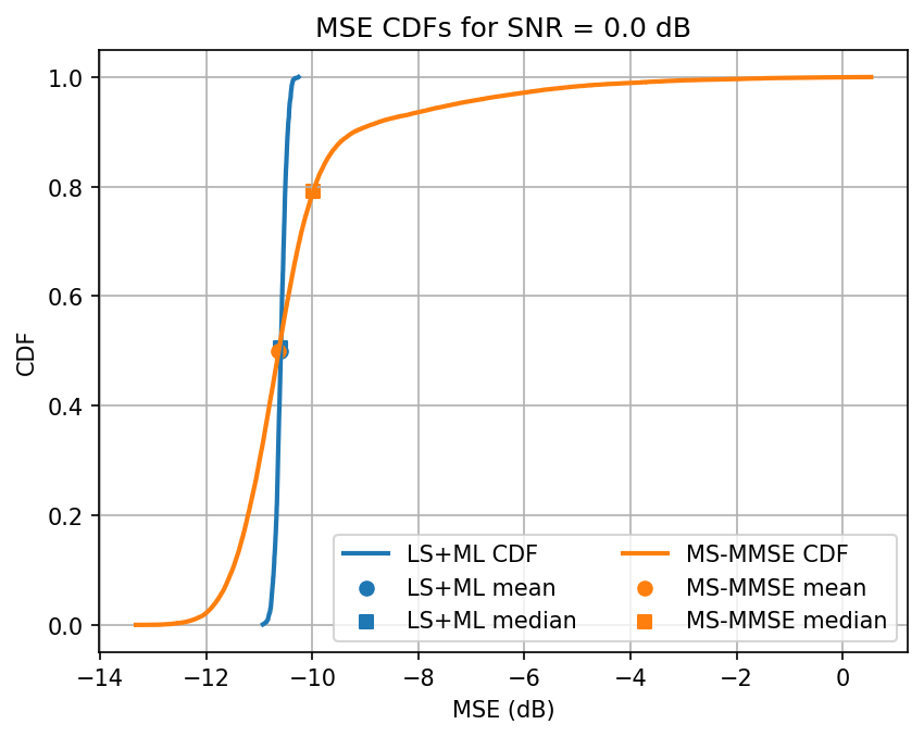
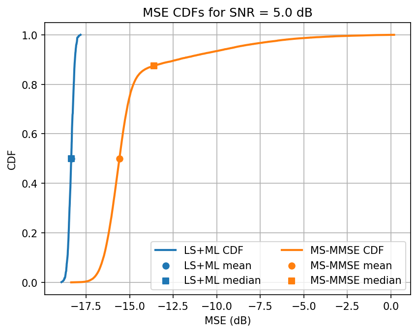
# Plot CDFs of MSE losses
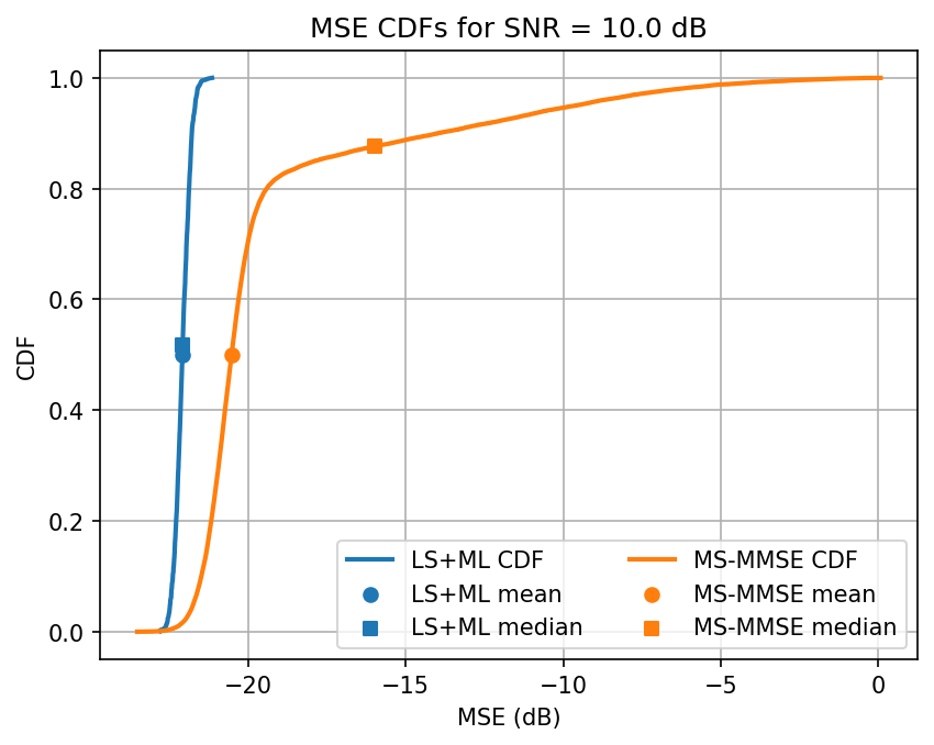
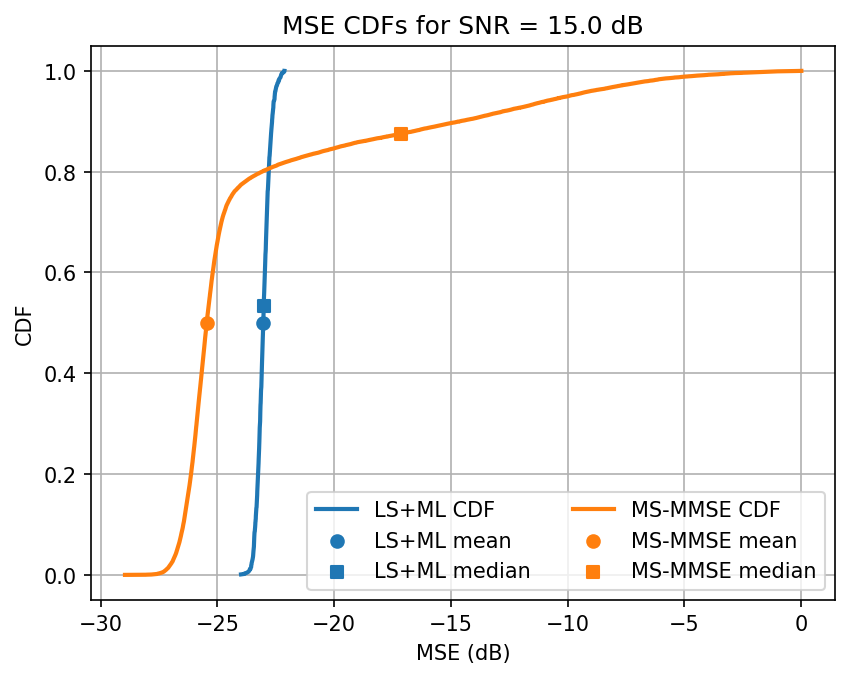
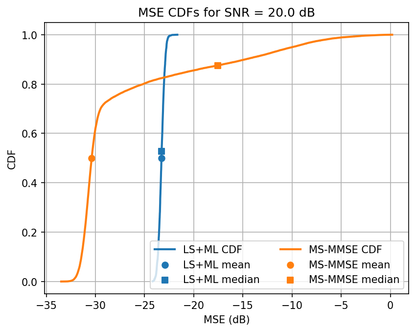
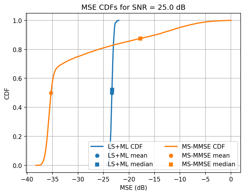
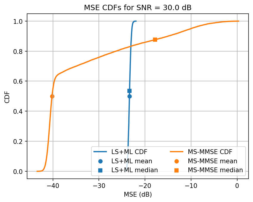
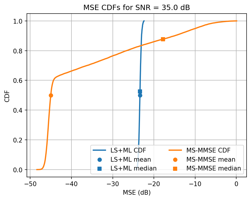
ut.plot_annotaded_cdfs([ml_loss, mmse_loss_pyaerial], ['LS+ML', 'MS-MMSE'],
title=f'MSE CDFs for SNR = {snr} dB')
XLA can lead to reduced numerical precision. Use with care.
Testing SNR -10.0 dB
Testing model trained on SNR 10
Testing LS & MS-MMSE in PyAerial: 100%|█████████████████████████████████████████████████████████████████████████████████| 1000/1000 [01:11<00:00, 14.01it/s]
Avg. ML test loss for -10.0 dB SNR is 3.2 dB
Testing SNR -5.0 dB
Testing model trained on SNR 10
Testing LS & MS-MMSE in PyAerial: 100%|█████████████████████████████████████████████████████████████████████████████████| 1000/1000 [00:46<00:00, 21.36it/s]
Avg. ML test loss for -5.0 dB SNR is -3.0 dB
Testing SNR 0.0 dB
Testing model trained on SNR 10
Testing LS & MS-MMSE in PyAerial: 100%|█████████████████████████████████████████████████████████████████████████████████| 1000/1000 [00:47<00:00, 21.25it/s]
Avg. ML test loss for 0.0 dB SNR is -10.6 dB
Testing SNR 5.0 dB
Testing model trained on SNR 10
Testing LS & MS-MMSE in PyAerial: 100%|█████████████████████████████████████████████████████████████████████████████████| 1000/1000 [00:46<00:00, 21.39it/s]
Avg. ML test loss for 5.0 dB SNR is -18.4 dB
Testing SNR 10.0 dB
Testing model trained on SNR 10
Testing LS & MS-MMSE in PyAerial: 100%|█████████████████████████████████████████████████████████████████████████████████| 1000/1000 [00:46<00:00, 21.33it/s]
Avg. ML test loss for 10.0 dB SNR is -22.1 dB
Testing SNR 15.0 dB
Testing model trained on SNR 10
Testing LS & MS-MMSE in PyAerial: 100%|█████████████████████████████████████████████████████████████████████████████████| 1000/1000 [00:46<00:00, 21.39it/s]
Avg. ML test loss for 15.0 dB SNR is -23.0 dB
Testing SNR 20.0 dB
Testing model trained on SNR 10
Testing LS & MS-MMSE in PyAerial: 100%|█████████████████████████████████████████████████████████████████████████████████| 1000/1000 [00:46<00:00, 21.36it/s]
Avg. ML test loss for 20.0 dB SNR is -23.3 dB
Testing SNR 25.0 dB
Testing model trained on SNR 10
Testing LS & MS-MMSE in PyAerial: 100%|█████████████████████████████████████████████████████████████████████████████████| 1000/1000 [00:46<00:00, 21.38it/s]
Avg. ML test loss for 25.0 dB SNR is -23.3 dB
Testing SNR 30.0 dB
Testing model trained on SNR 10
Testing LS & MS-MMSE in PyAerial: 100%|█████████████████████████████████████████████████████████████████████████████████| 1000/1000 [00:46<00:00, 21.36it/s]
Avg. ML test loss for 30.0 dB SNR is -23.4 dB
Testing SNR 35.0 dB
Testing model trained on SNR 10
Testing LS & MS-MMSE in PyAerial: 100%|█████████████████████████████████████████████████████████████████████████████████| 1000/1000 [00:46<00:00, 21.39it/s]
Avg. ML test loss for 35.0 dB SNR is -23.4 dB
Testing SNR 40.0 dB
Testing model trained on SNR 10
Testing LS & MS-MMSE in PyAerial: 100%|█████████████████████████████████████████████████████████████████████████████████| 1000/1000 [00:46<00:00, 21.36it/s]
Avg. ML test loss for 40.0 dB SNR is -23.3 dB
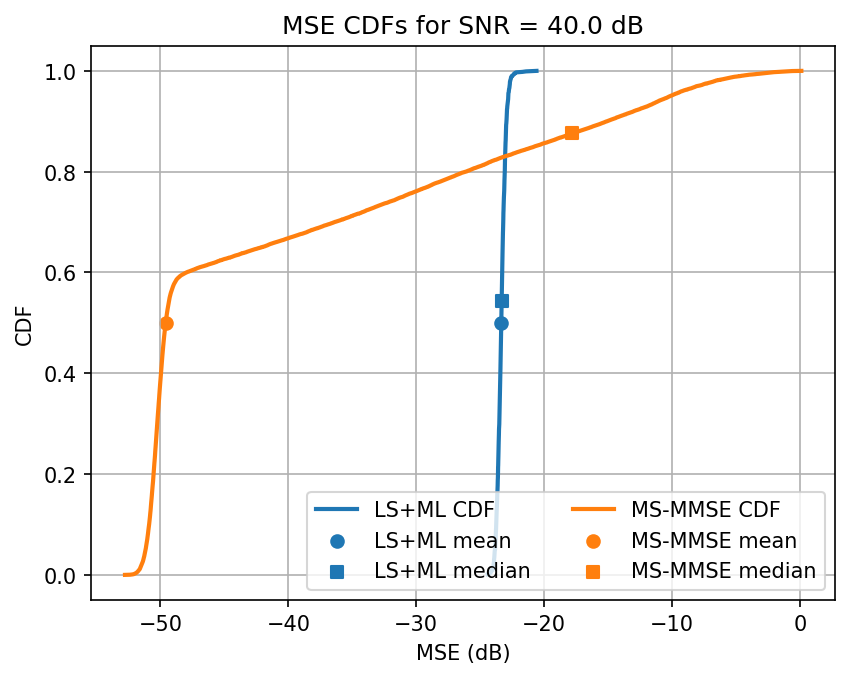
观察:当我们微调训练时,我们看到 ML 模型在大多数 SNR 下优于 MS-MMSE 方法。当需要插值时,性能略有下降。此外,对于更广泛的信道类别,ML 似乎更可靠。对于 ML,估计的方差较低,平均而言,即使中位数继续衰减,其性能在高 SNR 下也会饱和。
跨 SNR 绘制比较图#
要求:test_snrs 必须包含多个元素。请阅读下文,了解我们为什么要这样做。
取决于 SNR 的模型切换:信道估计中的挑战之一是使其跨 SNR 工作。较低的 SNR 具有较高的信道估计均方误差 (MSE),这更严重地影响了这些样本在机器学习模型中的损失,从而导致模型仅学习低 SNR 信道。避免此问题的一种方法是进行模型切换方法。在模型切换中,每个模型都针对单个 SNR 进行训练,并使用 SNR 最接近用户 SNR 的模型。
请注意,此方法需要对 SNR 进行足够好的估计,以便选择正确的模型。通常,获取这样的估计并不困难 - 例如,使用 MMSE 信道估计应该具有比需要的更高的分辨率。因此,这里我们假设用户的 SNR 是已知的,并且选择了最接近的模型。
如果我们设置 train_snrs = [-10, 0, 10, 20, 30, 40] 和 test_snrs = [-10, -5, 0, 5, 10, 15, ..., 40],那么我们将看到为 -10 dB 的 SNR 训练的模型也用于估计 -5 dB 的信道,并且为 0 dB 训练的模型也用于 5 dB 等。这导致 SNR 可被 5 但不能被 10 整除时,MSE 较高。
[4]:
plt.figure(dpi=200)

plt.plot(test_snrs, snr_losses_ls,              '-', label='LS',                     color ='k', alpha=.7)
plt.plot(test_snrs, snr_losses_ls_pyaerial,    '--', label='LS PyAerial',            color ='k')
plt.plot(test_snrs, snr_losses_ml,              '-', label='LS+ML (mean)',           color ='tab:orange')
plt.plot(test_snrs, snr_losses_ml2,            '--', label='LS+ML (median)',         color ='tab:orange')
plt.plot(test_snrs, snr_losses_mmse_pyaerial,   '-', label='MMSE PyAerial (mean)',   color ='tab:green')
plt.plot(test_snrs, snr_losses_mmse_pyaerial2, '--', label='MMSE PyAerial (median)', color ='tab:green')

plt.xlabel('SNR [dB]')
plt.ylabel('NMSE [dB]')
plt.xlim((min(test_snrs), max(test_snrs)))
plt.legend(fontsize=7)
plt.grid()
plt.show()
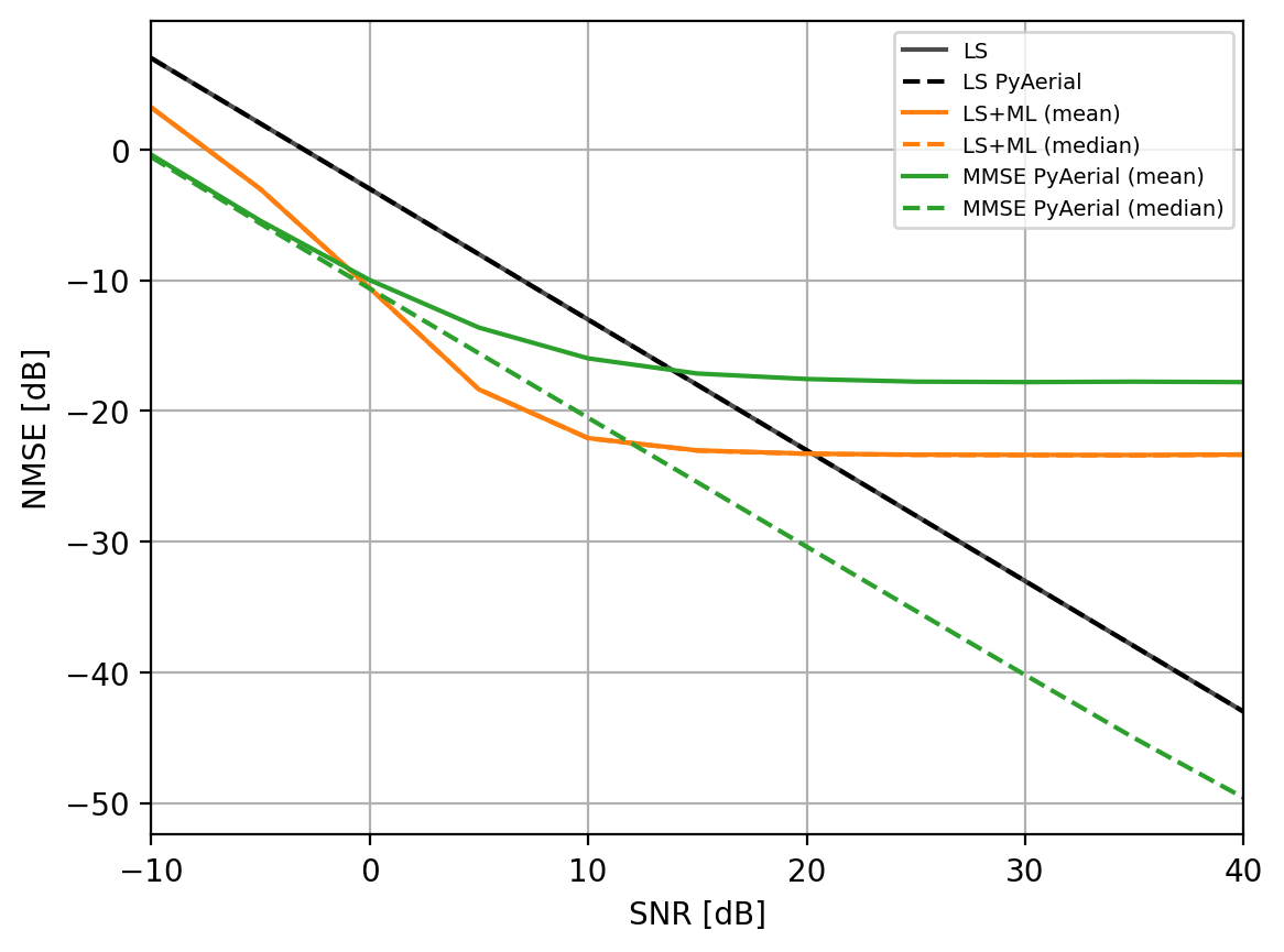
下面是 interp = 2 和 48 个 PRB 情况下的此图示例。
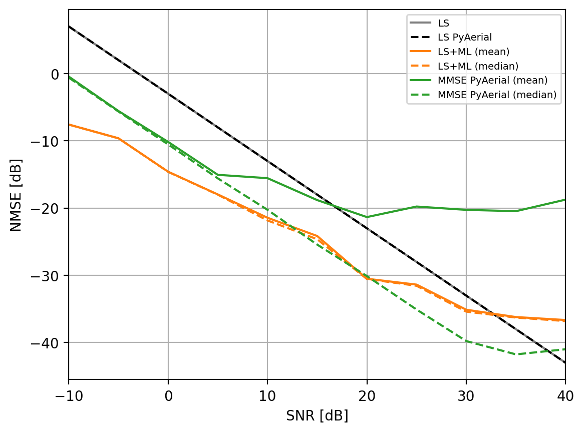
与 MS-MMSE 相比,一些值得注意的增益
对于 SNR \(\in [-10, 0]\) dB 的 5-8 dB 增益
对于 SNR \(\in [ 0, 10]\) dB 的 3-5 dB 增益
对于 SNR \(\in [10, 20]\) dB 的 0-3 dB 增益
在 10 dB 之后,ML 模型相对更可靠,具有更可预测的 CDF 和更好的平均性能
请注意,此方法有望在更高的 PRB 分配下更好地工作。可能是由于能够从信道中提取更多信息。当 interp = 1 时,该模型也具有更好的性能,因为不需要插值,这使得网络通过在末尾添加全连接层而更难训练。
实际部署的注意事项#
为了使这种方法在实际部署中工作,它需要两个额外的步骤,为了简单起见,我们在此处省略了这两个步骤
SNR 估计:需要估计优化的模型以执行信道估计。在这里,我们认为 SNR 是已知的。
PRB 并行化:在推理期间,PRB 并行器会将 LS 估计值(例如 78 个 PRB)拆分为多个块,这些块可以由不同大小的训练模型并行处理,然后再重新组合在一起。例如,如果我们为 {1, 4, 16} PRB 训练模型,则 78 PRB 估计值将导致 16 PRB 模型 4 个批次,4 PRB 模型 3 个批次和 1 PRB 模型 2 个批次(4 * 16 + 3 * 4 + 2*1 = 64 + 12 + 2 = 78)
在 Aerial Omniverse Digital Twin 中评估系统级性能#
本笔记本可用于生成与 AODT 中 PUSCH 信道估计的机器学习示例兼容的模型。只要 models_folder 变量在多次运行中保持不变,单个文件夹将被填充用于多个 SNR 和 PRB 的正确结构。正如 AODT 用户指南中所述,然后需要将此文件夹移动到 AODT 后端可访问的目录,并将 config_est.ini 文件填充文件夹的绝对路径。
使用 PyAerial 作为 AODT 桥梁的优势
AODT 使用高性能 EM 求解器来计算射线追踪传播仿真。射线追踪对于研究特定于站点的设置中的 ML 方法是必要的,为以前在随机仿真中不可用的边缘情况提供洞察力和可解释性。
AODT RAN 仿真使用与现实世界中部署的硬件相同的软件运行。这种前所未有的组合创建了准确的系统表示,使研究人员有可能设计新功能(无论是否由 AI/ML 驱动)并评估其全网端到端的影响。
PyAerial 目前仅为 cuPHY(Aerial 的 PHY 层)提供 Python 接口。因此,PyAerial 中无法进行超出 PHY 的比较,并且可以计算的最后一个链路级量是误块率。另一方面,AODT 集成了 Aerial 的 cuPHY 和 cuMAC,使研究人员能够衡量信道估计如何影响更高层。
有关如何在 AODT 中运行此 ML 信道估计的更多信息,请参阅 AODT 用户指南。