计算和绘制 TTS 数据集中音素的分布#

在本教程中，我们将使用参考文本语料库分析 ljspeech 文本语料库的音素分布。参考语料库被假定为具有正确的音素分布。

我们的分析将包括创建参考和样本音素分布的条形图。其次，我们还将计算 ljspeech 音素分布与参考分布相比的差异。

安装所有必需的软件包。

!pip install bokeh cmudict prettytable nemo_toolkit['all']
!pip install protobuf==3.20.0

# Put all the imports here for ease of use, and cleanliness of code 
import os
import pprint
import json
# import nemo g2p class for grapheme to phoneme
from nemo_text_processing.g2p.modules import EnglishG2p

# Bokeh
from bokeh.io import output_notebook, show
from bokeh.plotting import figure, output_file, show
from bokeh.io import curdoc, export_png
from bokeh.models import NumeralTickFormatter
output_notebook()

from prettytable import PrettyTable

# Counter 
import collections
from collections import Counter

pp = pprint.PrettyPrinter(indent =4, depth=10)

获取 arpabet 文件#

从 nemo 获取 CMU 字素到音素字典。

!wget https://raw.githubusercontent.com/NVIDIA/NeMo/v1.12.0/scripts/tts_dataset_files/cmudict-0.7b_nv22.08

创建 g2p 对象。此对象将在整个过程中用于将字素转换为音素

g2p = EnglishG2p(phoneme_dict="cmudict-0.7b_nv22.08", ignore_ambiguous_words=False)

参考分布：#

我们将使用不仅涵盖英语中每个音素（共有 44 个），而且还表现出与英语相同的频率分布的参考分布。因此，我们可以使用此参考分布来比较其他数据集的音素分布。这使得能够识别数据中的差距，例如需要更多具有特定音素的样本。

我们将使用 NeMo 字素到音素将单词转换为音素。
列出 g2p 字典中的所有音素

# create a list of the CMU phoneme symbols
phonemes = {k: v[0] for k, v in g2p.phoneme_dict.items()}
pp.pprint(list(g2p.phoneme_dict.items()))

加载参考分布#

我们将加载参考频率分布并在本节中将其可视化。

ref_corpus_file = "text_files/phoneme-dist/reference_corpus.json"
with open(ref_corpus_file) as f:
    freqs_ref = json.load(f)

让我们看一下参考分布

freqs_ref =dict(sorted(freqs_ref.items()))

xdata_ref = list(freqs_ref.keys())
ydata_ref = list(freqs_ref.values())

pp.pprint(freqs_ref)

绘制参考频率分布

p = figure(x_range=xdata_ref, y_range=(0, 5000), plot_height=300, plot_width=1200, title="Reference phoneme frequency distribution",toolbar_location=None, tools="")

curdoc().theme = 'dark_minimal'

# Render and show the vbar plot
p.vbar(x=xdata_ref, top=ydata_ref)

# axis titles 
p.xaxis.axis_label = "Arpabet phonemes"
p.yaxis.axis_label = "Frequency of occurrence"

# display adjustments 
p.title.text_font_size = '20px'
p.xaxis.axis_label_text_font_size = '18px'
p.yaxis.axis_label_text_font_size = '18px'
p.xaxis.major_label_text_font_size = '6px'
p.yaxis.major_label_text_font_size = '18px'

show(p)

现在编写一个函数来获取文本语料库的词频。

def get_word_freq(filename):
    """
        Function to find phoneme frequency of a corpus.
        arg: filename: Text corpus filepath.
        return: frequencies of every phoneme in the file.
    """
    freqs = Counter()
    with open(filename) as f: 
        for line in f: 
            for word in line.split(): 
                freqs.update(phonemes.get(word, [])) 
    return freqs

样本语料库音素#

我们将查看来自 ljspeech 数据集的文本的音素分布。本教程我们不需要 LJspeech wav 文件。因此，为简单起见，我们可以使用 text_files/phoneme-dist/Ljspeech_transcripts.csv 中的 Ljspeech 成绩单文件

从 Ljspeech_transcripts.csv 中删除 wav 文件名以生成 Ljspeech 文本语料库。

!awk -F"|" '{print $2}' text_files/phoneme-dist/Ljspeech_transcripts.csv > ljs_text_corpus.txt

加载 Ljspeech 文本语料库文件并创建音素的频率分布。
我们将使用 NeMo 字素到音素将单词转换为 cmu 音素。

in_file_am_eng = 'ljs_text_corpus.txt'
freqs_ljs = get_word_freq(in_file_am_eng)

# display frequencies
freqs_ljs=dict(sorted(freqs_ljs.items()))

xdata_ljs = list(freqs_ljs.keys())
ydata_ljs = list(freqs_ljs.values())

pp.pprint(freqs_ljs)

让我们像对参考分布所做的那样绘制 ljspeech 语料库的频率分布。

p = figure(x_range=xdata_ljs, y_range=(0, 70000), plot_height=300, plot_width=1200, title="Phoneme frequency distribution of ljspeech corpus",toolbar_location=None, tools="")

curdoc().theme = 'dark_minimal'

# Render and show the vbar plot
p.vbar(x=xdata_ljs, top=ydata_ljs)

# axis titles 
p.xaxis.axis_label = "Arpabet phonemes"
p.yaxis.axis_label = "Frequency of occurrence"

# display adjustments 
p.title.text_font_size = '20px'
p.xaxis.axis_label_text_font_size = '18px'
p.yaxis.axis_label_text_font_size = '18px'
p.xaxis.major_label_text_font_size = '6px'
p.yaxis.major_label_text_font_size = '18px'

show(p)

一起绘制分布#

我们将需要 CMU 字典符号的规范列表，并且需要知道该列表的长度与我们的语料库相比如何。

CMU phones:  
['AA0', 'AA1', 'AA2', 'AE0', 'AE1', 'AE2', 'AH0', 'AH1', 'AH2', 'AO0', 'AO1', 'AO2', 'AW0', 'AW1', 'AW2', 'AY0', 'AY1', 'AY2', 'B', 'CH', 'D', 'DH', 'EH0', 'EH1', 'EH2', 'ER0', 'ER1', 'ER2', 'EY0', 'EY1', 'EY2', 'F', 'G', 'HH', 'IH0', 'IH1', 'IH2', 'IY0', 'IY1', 'IY2', 'JH', 'K', 'L', 'M', 'N', 'NG', 'OW0', 'OW1', 'OW2', 'OY0', 'OY1', 'OY2', 'P', 'R', 'S', 'SH', 'T', 'TH', 'UH0', 'UH1', 'UH2', 'UW0', 'UW1', 'UW2', 'V', 'W', 'Y', 'Z', 'ZH']

arpa_list = g2p.phoneme_dict.values()
cmu_symbols = set()
for pronunciations in arpa_list:
    for pronunciation in pronunciations:
        for arpa in pronunciation:
            cmu_symbols.add(arpa)
cmu_symbols = list(cmu_symbols)
cmu_symbols.sort()
print(cmu_symbols)

将两个分布组合在一起。

data_combined = dict.fromkeys(cmu_symbols, 0)

for key in cmu_symbols: 
    if key in freqs_ref: 
        data_combined[key] += freqs_ref[key]
    if key in freqs_ljs: 
        data_combined[key] += freqs_ljs[key]

xdata_combined = list(data_combined.keys())
ydata_combined = list(data_combined.values())

pp.pprint(data_combined)

音素与参考分布的比较#

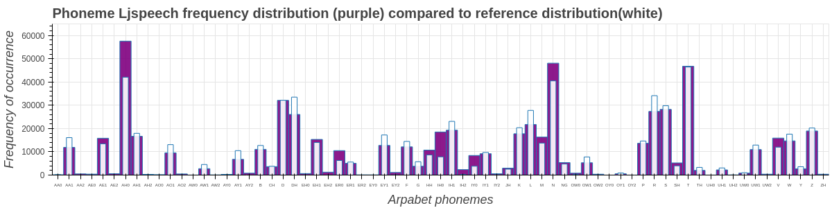
为了进行分析，我们现在将一起查看两个分布。

首先，我们要将参考分布缩放到 LJs 分布。获取 Ljspeech 分布中的总音素和总参考分布音素，并计算缩放因子，然后缩放参考分布音素量以匹配 Ljspeech 分布，然后绘制参考音素分布与 Ljspeech 音素分布的对比图。

# get the total phonemes in the reference phonemes 
ref_total = sum(freqs_ref.values())

# get the total phonemes in the comparison dataset
ljs_ph_total = sum(freqs_ljs.values())

# The scale factor is: 
scale_ljs = ljs_ph_total / ref_total

scaled_for_ljs = {} 
for phonemes in freqs_ref.items(): 
    scaled_for_ljs[phonemes[0]] = int(phonemes[1] * scale_ljs)
    

xscaled_for_ljs = list(scaled_for_ljs.keys())
yscaled_for_ljs = list(scaled_for_ljs.values())

一起绘制两个分布

p = figure(x_range=xdata_combined, y_range=(0, 65000), plot_height=300, plot_width=1200, title="Phoneme Ljspeech frequency distribution (purple) compared to reference distribution(white)",toolbar_location=None, tools="")

curdoc().theme = 'dark_minimal'

# Render and show the vbar plot - this should be a plot of the comparison dataset
p.vbar(x=xdata_ljs, top=ydata_ljs, fill_alpha=0.9, fill_color='purple')

# Render a vbar plot to show the reference distribution
p.vbar(x=xscaled_for_ljs, top=yscaled_for_ljs, fill_alpha=0.9, fill_color='white', width=0.5)

# axis titles 
p.xaxis.axis_label = "Arpabet phonemes"
p.yaxis.axis_label = "Frequency of occurrence"

# display adjustments 
p.title.text_font_size = '20px'
p.xaxis.axis_label_text_font_size = '18px'
p.yaxis.axis_label_text_font_size = '18px'
p.xaxis.major_label_text_font_size = '6px'
p.yaxis.major_label_text_font_size = '12px'
p.yaxis.formatter = NumeralTickFormatter(format="0")

show(p)

计算参考分布和总音素之间的主要差异#

在这里，我们将检查每个音素的两个语料库之间在数量和百分比上的差异。

diff_combined = {} 
for phonemes in data_combined.items():
    if phonemes[0] in scaled_for_ljs : 
        difference = phonemes[1] - scaled_for_ljs[phonemes[0]]
        min_ = min(phonemes[1], scaled_for_ljs[phonemes[0]])
        max_ = max(phonemes[1], scaled_for_ljs[phonemes[0]])
        percentage = round(((1 - (min_ / max_)) * 100), 2)
        diff_combined[phonemes[0]] = (difference, percentage)       
    else : 
        diff_combined[phonemes[0]] = (0,0)

t = PrettyTable(['Phoneme', 'Difference in volume', 'Difference in percentage'])
for phonemes in diff_combined.items() : 
    t.add_row([phonemes[0], phonemes[1][0], phonemes[1][1]])
print(t)

结论#

在本教程中，我们了解了如何分析数据的音素分布。我们可以使用本教程中解释的技术来查找数据集中需要更多表示的任何音素。本教程之后应平衡数据的音素分布。这可以通过添加更多包含覆盖率较低的音素的句子来实现。

NVIDIA Riva

计算和绘制 TTS 数据集中音素的分布

目录